LM – Curve Derivation with Diagram

What is the LM Curve?

• L = Liquidity demand (money demand)
• M = Money supply

The LM Curve shows the relationship between interest rate {r} and income/output (y) when the money market is in equilibrium. So, the LM curve represents the various combinations of interest rate and income (r & y) required to maintain the money market equilibrium (M^d = M^s).

To derive the LM curve, money demand is assumed to be a positive function of income and a negative function (inverse) of the interest rate. Both transaction and precautionary demand for money are positive functions of income, and speculative demand for money is an inverse function of interest rate. So, a simple linear form of the  money demand function can be written as

Md = a_o + a₁Y – a₂r ———- (i)

Where,

• a_o = autonomous money demand, a_o >0
• a₁ = income sensitivity of money demand, a1 > 0
• a₂ = interest sensitivity of money demand, a₂ > 0

Money supply is assumed to be the policy choice variable, which depends on the policy of the central bank, and it is given.

i.e M^s = M_o ————(ii)

Where Mo = given money supply

Now, the money market is said to be in equilibrium when both money demand and money supply are equal.

i.e. M^d = M^S

Or, a_o + a₁Y – a₂r = M_o  (from equations (i) and (ii)

Or, – a₂r = – ao + M_{o –} a₁Y

Or,  a₂r = ao – M_{o  +} a₁Y

r= (a_o – M_o)  _/ a_{2   +}  a_1/ a_2. Y  ————– (iii)

This equation (iii) shows the relationship between r and Y when the money market is in equilibrium. So, this equation (iii) itself represents the LM curve with the intercept (a_o – M_o)  _/ a₂   and slope a_1/ a_2.

As a₁ >0 and a₂ > 0, the slope of the LM curve is positive or upward sloping, and it depends on the two parameters a₁ & a_2.

If the income sensitivity of money demand a₁ is higher than the interest sensitivity a_{2, the} LM curve will be steeper and less elastic.

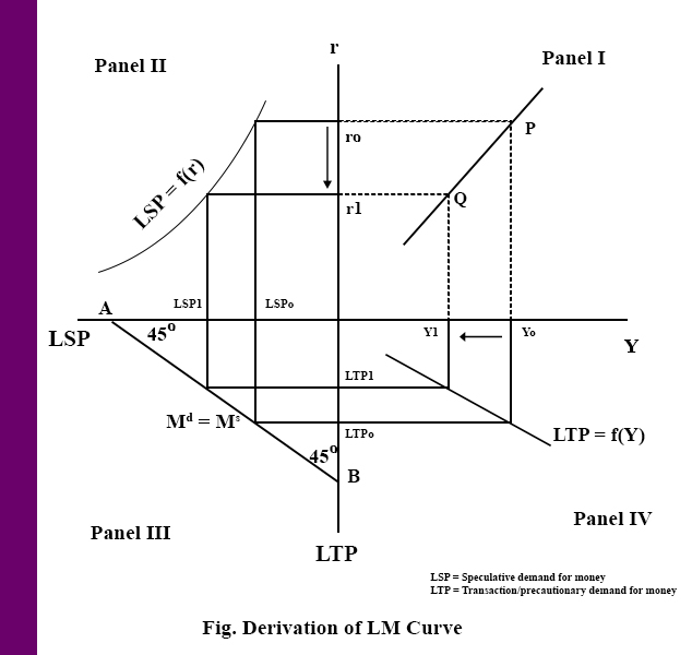
Here,

• Panel (II) speculative money demand function
• Panel (III) money market equilibrium
• Panel (IV) shows the transaction and precautionary money demand function
• Panel (I) shows the LM curve with the help of other panels.

As in panel (I), if the interest rate is r_o, the speculative demand for money is LSP_o. As the money supply is given, the transaction and precautionary demand for money should be LTP_o. Thus, LSPo + LTPo = Ms, as shown in panel (II).

Similarly, for LTPo amount of transaction and precautionary demand for money, income should be Y_o, which is shown in panel (III). It means if the interest rate is r0 and the income is Yo, the money market is in equilibrium, where point P in panel (IV) represents this specific combination of r and Y.

Similarly, the point Q in panel (IV) indicates that the money market is in equilibrium when the interest rate is r1 and the income is Y1. If we join these points P and Q in panel (IV), we get the positively sloped curve known as the LM-curve.

Shifts of the LM Curve

• Changes in Money Supply (MS)
• Increase in Money Supply (Ms ↑) caused by expansionary monetary policy (e.g., open market purchase, lower CRR/SLR, lower policy rate). → LM curve shifts rightward / downward
• Decrease in Money Supply (Ms ↓) caused by contractionary monetary policy (e.g., open market sale, higher CRR/SLR, higher policy rate). → LM curve shifts leftward / upward
• Changes in Price Level (P)
• Increase in Price Level (P ↑) → LM curve shifts leftward / upward
• Decrease in Price Level (P ↓) → LM curve shifts rightward / downward

General equilibrium under the IS-LM Framework

Under the IS-LM framework, the general equilibrium is defined as the situation in which both the real sector and the monetary sector are simultaneously in equilibrium. It means the specific combination of the interest rate and income represents a general equilibrium at which both the real and monetary sector attains equilibrium at the same time.

The real sector equilibrium is represented by the IS curve, which is downward sloping, and the monetary sector equilibrium is represented by the LM curve, which is upward sloping. So, the point of intersection between the IS and LM curves determines the general equilibrium.

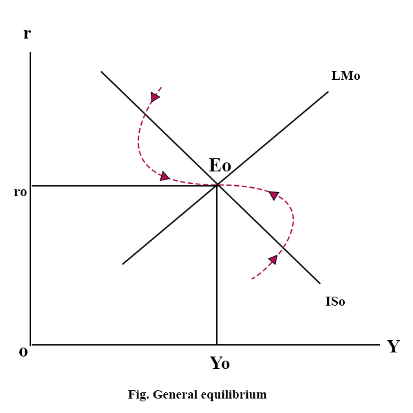
Here, both real and monetary sector equilibrium is given by point Eo, which means the economy attains general equilibrium at the optimal interest rate and Oyo output/income.

Such an equilibrium under the IS-LM model is said to be stable because the disturbances in the equilibrium are only temporary, and sooner or later, the economy attains this equilibrium.

There is an inherent mechanism in both the real and monetary sectors that brings the economy back into equilibrium. This disequilibrium in the real sector adjusts income or output, whereas the financial sector disequilibrium gradually adjusts the interest rate, and the economy reaches equilibrium.