- Developed independently by Roy F. Harrod in 1939 and Evsey Domar in 1946.
- Harrod–Domar growth model is one of the Keynesian models of economic growth.
| Increase | Result | Term |
|---|---|---|
| Income (Y) ↑ | Investment (I) ↑ | Accelarator |
| Investment (I) ↑ | Income (Y) ↑ | Multiplier |
The H-D growth model is the dynamic extension of the Keynesian income and output determination model developed by Roy F. Harrod (1939) and Evsey Domar (1946). Since the basic framework, analysis, and conclusion of both are similar and so we often consider them as a single H-D growth model.
The H-D growth model shows that the interaction between the multiplier and accelerator produces economic growth, and this model finds the optimum growth that maintains the equilibrium of the economy.
i.e. Aggregate Demand (AD) = Aggregate Supply (AS)
It means this model helps to find the required growth rate of income and output in order to keep the economy in equilibrium. Furthermore, this model explains what happens if such a required growth rate is not achieved.
Basic Assumptions of the H-D Growth Model
1) There are two inputs: capital (K) and labor (L), which are combined in a fixed proportion.
2) Technology is constant, and there is a constant return to scale in production.
3) The economy is of two sectors, where the household sector makes consumption, and the business sector invests.
4) The household sector consumer some part of their income and save the remaining part.
5) The aggregate saving of the economy (S) is a constant proportion of income or output of the same period.
i.e. S = s.Y ——– (i)
Where,
- S = Aggregate saving
- s = saving rate or MPS 0<s<1
- Y = income or output
6) Investment is determined by the acceleration principle, and investment is constant times the change in output from the previous period.
i.e. I = v.Δ Y ———- (ii)
Where,
- I = Investment
- v = acceleration coefficient or capital output rate, v > 0
- Δ Y = change in output
7) Labor supply is growing at a constant rate determined exogenously.
i.e. Growth rate of labor supply = λ (λ = 2.1 भनेको Labout supply 21% ले बढ्यो भनेको हो )
Based on these assumptions, this model finds the growth rate of income and output required to keep the economy in equilibrium. In this two-sector economy, it is said to be in equilibrium when investment and saving are equal.
i.e. I = S
- or, v.Δ Y = s.Y (from equations i and ii)
- or, Δ Y/Y = s/v ———– (iii)
This equation (iii) shows that for the equilibrium of the economy (I = S), income should grow at the rate of s/v, which is called the warranted or required growth rate in this model. It means the income or output is required to grow by s/v to maintain the economy in equilibrium.
However, the economy may not be able to achieve such a warranted (required) growth rate. To explain the dynamic stability of the equilibrium, this model defines three different growth rates and analyzes them.
A) Actual growth rate (Ga): It is the growth rate realized by the economy, and is given by Ga = s/Va. Where, S = saving rate or MPS, Va = actual capital output ratio
B) Warrented Growth Rate (Gw): It is the growth rate required to maintain the equilibrium of the economy. It is assumed that this growth rate is required to fully utilize the capacity of the economy and satisfy the business people’s expectations. It is given by Gw = s/Vw.
Vw = warranted/expected/required capital output ratio
C) Natural growth rate (Gn): It is the long-run equilibrium growth rate of the income or output of the economy. It is argued that in the long run, the economy is growing at the rate of growth of labor supply. i.e. Gn = λ.
For the dynamic stability of the economy, all of these growth rates should be equal simultaneously.
i.e. Ga = Gw = Gn
However, there are two fundamental problems in this model, which are
- Problem of attaining equilibrium
- Problem of maintaining equilibrium
The first fundamental problem occurs because all three growth rates are determined independently by the different sectors of the economy.
For example,
- Ga = depends on the saving rates (S) and the actual capital output ratio (Va). Where S depends on the behavior of the general public, and Va depends on the actual state of technology and the business environment.
- Gw = depends mainly on the business people’s expectations.
- Gn = depends on the demographic factors such as the size of the population, labor force participation rate, migration, etc.
Since these different factors are determined by the different sectors, and there is a remote chance that all of them (Ga, Gw, Gn) converged to each other and make all of these growth rates equal simultaneously. If it happens, then it is a happy accident as called by Robinson.
The second problem is to maintain the equilibrium because if the equilibrium is disturbed due to any reason, then it is impossible to regain the equilibrium.
The economy either moves to hyperinflation or depression, ultimately, if the equilibrium is disturbed.
When actual growth rate increases after some time
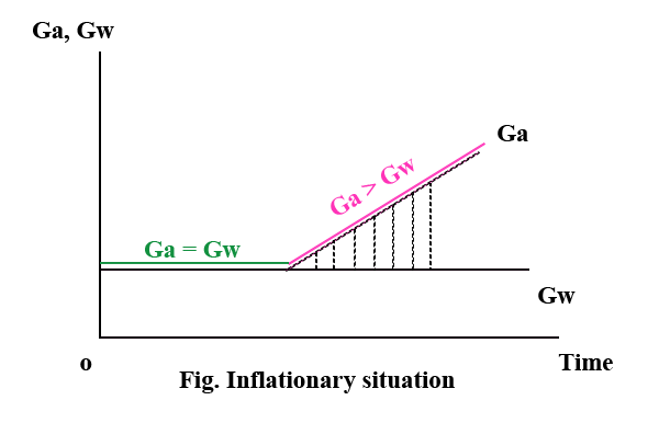
The economy is growing faster than the expectations of the business people, and there are shortages of capacity in the economy. This motivates the private sector to make more investments, which increases the actual growth rate. Since Ga is already higher than Gw, this increases the gap between Ga and Gw further.
i.e. Ga >> Gw
This results in inflationary pressure in the economy, and ultimately, the economy experiences hyperinflation.
When actual growth rate decreases after some time
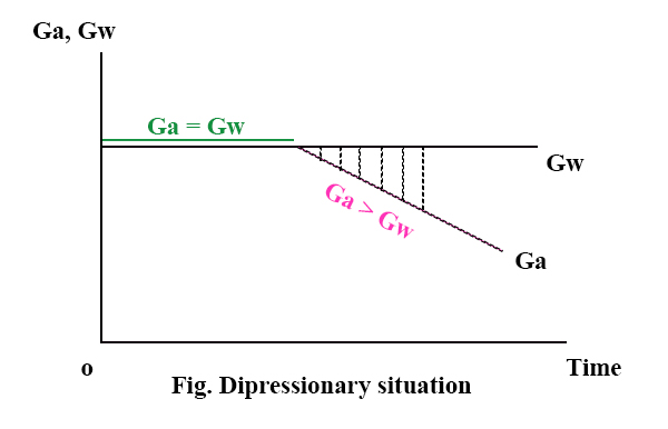
If Ga < Gw, then the economy is growing slower than the productive capacity (supply capacity), indicating underutilization of the capacity. This discouraged the private sector from reducing the investments, which lowers the Ga. Since Ga is already lower than Gw, the gap between them further increases (i.e. Ga <<< Gw), and the economy ultimately falls into depression.
This shows that the equilibrium under the H-D growth model is highly unstable. No matter what the small disturbances in the equilibrium, the economy moves to either hyperinflation or depression. So, this model is said to rest on the Razor’s edge (knife’s edge) equilibrium.
Uses of H-D Growth Model
- This model is widely used in developing countries in order to determine the growth target for the specific period. The targeted growth rate is estimated as growth rate = s/v
- This model can also be used to estimate the resource requirement to achieve the targeted growth rate. If such a growth rate is predetermined, then the resource requirement is estimated as resource requirement = Growth target (Gt) . v
- This model can help to prioritize the project and select the appropriate project to achieve the targeted growth from the given resources. For example, the project can be prioritized and selected based on its capital output ratio. The higher the capital output ratio, the higher the growth rate.
- This model helps the policy maker to identify the determinants of growth. The major determinants of the growth rate are saving, investment, capital output ratio (efficiency of capital), and labor supply.
Limitations of H-D Growth Model
- H-D growth model is seriously criticized both theoretically and empirically on the assumption of a fixed proportion of income, capital, and labor. The neoclassical growth theory shows that capital and labor can change over the period.
- This model can not explain the increasing returns to scale realized by most of the industrialized countries because of this model’s assumption of constant returns to scale.
- This model assumes constant technology, but in reality, the technology is changing over the period.
- The economy can not be on the razor’s edge as this model shows because the economy has some resilient capacity to adjust, and so if the equilibrium is disturbed, it is not necessary that the economy either falls into depression or hyperinflation.
Why H-D growth model is most commonly used in developing countries despite its limitations?
The H-D growth model has many limitations, but it is still more practiced in the developing countries by the policy makers due to the following reasons:
→ This model is easy to use and interpret, which makes this model commonly used. Under this model, we simply need the estimation of the savings and investment and the capital output ratio to estimate the growth rate.
→ There are data limitations in the developing countries which make it difficult for the use of other advanced modeling for growth estimation, such as computable general equilibrium (CGE), dynamic stochastic general equilibrium (DCGE), and macroeconomic models, etc.
→ H-D growth model is economic in terms of time, human resources, and financial resources, which makes the model more common in developing countries.
→ For the policymaker, estimation of the growth rate is an interest, and this H-D growth model can help direct estimation of the growth rate.
→ This model is used by the developing countries for growth rate estimation for the long term, and as a continuity of convention, this model is still in practice.
Other related posts