First read the ⇒ Collusive Oligopoly
Non-Collusive Oligopoly
In the non-collusive oligopoly market, firms do not have the information about the exact strategy of any of the rival firms. It is a situation like a non-cooperative game where each firm or player is using their own best strategy, assuming the strategy of others.
As there is no information about the exact strategy of rival firms, each of them assumes the strategy of response of the other and selects the best strategy to optimise their own objective, given the strategy of the other.
Each of the firms believes that they are using their best strategy under the given strategy of other firms. So, it gives a stable equilibrium known as the Nash Equilibrium (John Nash), but not the Pareto Efficient, which is possible only if there is collusion.
Based on the assumption regarding the behaviour of the rival firms, there are different models developed to explain the non-collusive oligopoly market. For example, the Cournot Model explains the non-collusive oligopoly market where each firm take their best output strategy assuming that the rival firms will keep their output constant at the previous level.
Similarly, the Bertrand Model considers that each firm decides their pricing strategy under the assumption that the rival firms keep their price at their previous level.
Though there are different alternative models to explain the non-collusive oligopoly market, the Kinked Demand Curve model developed by Paul Sweezy is considered a more realistic and representative model in the non-collusive oligopoly market.
According to Sweezy, the demand curve of a non-collusive oligopoly firm has a kink at the existing price and output.
This model argues that if the firm increases its price from the existing level, the other firms do not increase their price, and so the sales of the firm decline substantially because its product gets relatively expensive. This means the demand of the product above the existing price is more elastic or sensitive.
However, if the firm reduces the price from the existing level, the rival firms will also reduce their price in order to compete and retain their customers. So, the firm’s demand does not increase. Sufficiently, when it reduces the price from the existing level due to the follow of price reduction by others, this makes the part of the demand curve below the existing price less elastic or steeper. This difference in the price elasticity of demand between the two segments of the demand curve makes the demand curve kinked at the existing price and quantity.

Here, the demand curve of the firm is kinked at E, implying that P* and OQ* are the existing price and output. The part of the demand curve above the kinked point is flatter, indicating that the quantity demanded is more sensitive (elastic) to price, implying that if the firm increases the price from the existing price (P*) if affects the output.
Similarly, the part of the demand curve below P* is steeper or less elastic, implying that the quantity demanded is less elastic or sensitive to price if the firm reduces its price from P*; there is no significant impact on the output.
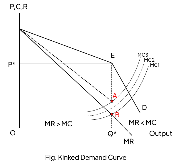
In this model, there is a gap in the marginal revenue curve (MR Curve), which is AB in the figure, due to the differences in elasticity between the two segments of the demand curve. Such a gap is higher if there are higher differences in the price elasticity between these two segments of the demand curve.
The marginal cost passes through this gap, and the price and output remain the same at the existing level. If the firm produces less than OQ*, then MR > MC, which means that by producing more, the firm can maximize profit. Similarly, if the firm produces more than OQ*, then MR<MC, which means it is better to reduce output. So, the existing price and output are the optimum or profit-maximizing for the firm. Since the existing price and output are optimal, or a profit-maximizing firm remains sticky (rigid) with the existing price and quantity.
This mode is said to be more realistic to explain the behavior of a non-collusive oligopoly market where the firms do not change their own cost because they have to compete with other rival firms. It means when the marginal cost of the firm changes due to any reason, but the other firms’ costs do not change, then the firm can not increase the price because if it increases the price, it will lose the market significantly as other firms are not increasing their price. So, a small change in marginal cost does not change the price of the firm. This model explains this behavior as the marginal cost within the gap of MR does not encourage the firm to change the price. The price and output can change only if the demand or cost of the whole industry changes.
Therefore, this model explains why price and output remains stickly in the non-collusive oligopoly market rather than explaining how price and output are determined. It shows that the price and output remain the same, though there may be a change in cost and demand of the individual firm, and the demand curve of the firm is kinked at the existing price and output.
Other posts