Demand Curve Derivation Using RPT
Revealed Preference Theory (RPT) can also be used to derive the demand curve, where the demand curve is derived by observing the actual behavior of the consumer under different price and income situations. If such a demand curve is derived by keeping money income constant, we obtain the Marshallian or Ordinary demand curve. If the demand curve is derived by keeping real income constant, we obtain the Slutsky demand curve in this approach. To explain such derivation of demand curve, assume that there are two commodities X and Y, and the price of the normal commodity X declines.
Derivation of demand curve for Normal good when Price decrease using RPT
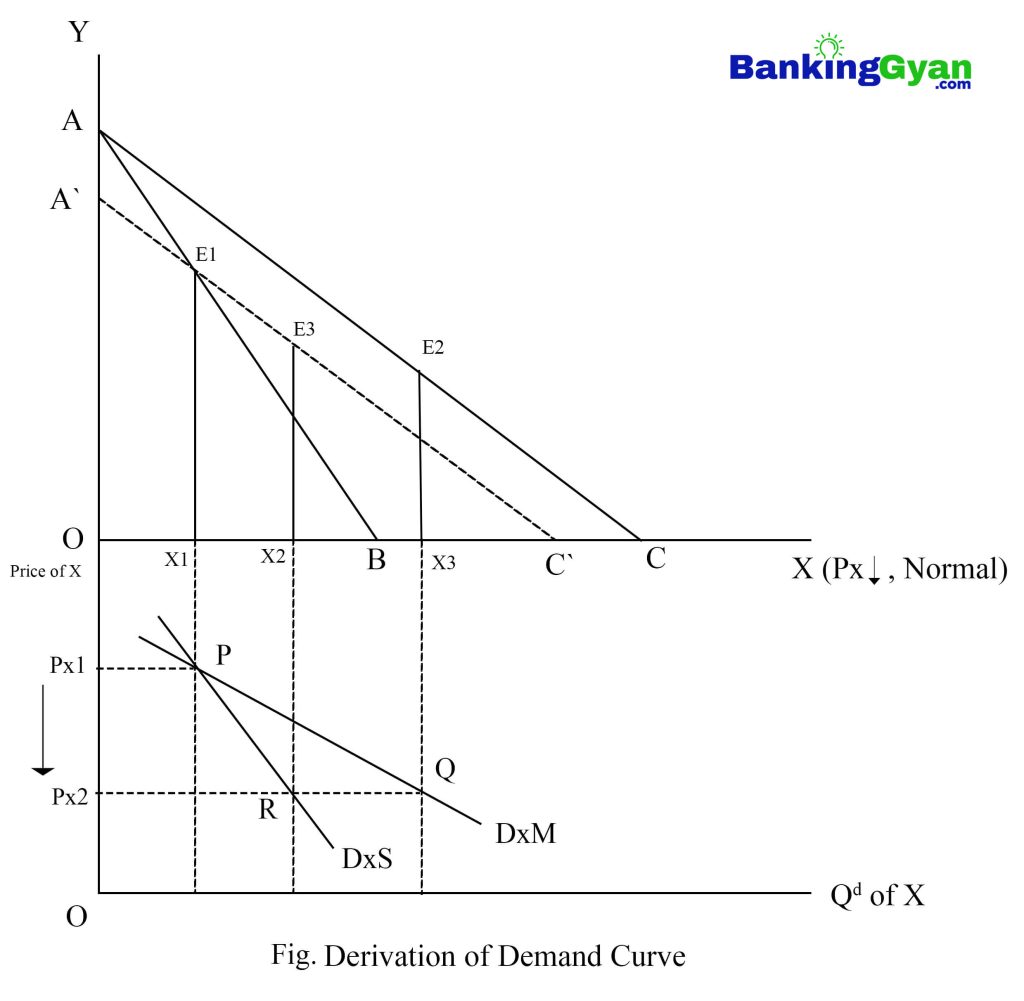
Here, AB is the initial budget line which means the consumer can select any bundle on this budget line or below of it. Being rational, the consumer does not select any bundle below the budget line and in order to find the actual selection of the consumer we have to observe his/her choice in the real market.
Now, assume that the consumer is found to be selecting E1 bundle, which consists of OX1 quantity of X. It means at the initial price Px1, the consumer demands OX1 quantity of X as shown by the point P in lower part of the figure.
Now, assume that price of X declines which swings the new budget line outward from AB to AB and consumer if observed to be selecting E2 bundle, which contains OX2 quantity of X. It means at the lower price Px2, the consumer demands OX2 quantity of X which is shown by point Q in the lower part of the figure. If we join the point P and Q then we get the ordinary or Marshallian demand curve (DxM).
This is downward sloping because it shows the price effect and price effect of normal goods is negative.
In order to derive the Slutskey or real income constant demand curve, we impose the tax to the consumer in such a way that the new budget line A`C` forms passing through the initial bundle E and parallel to the AC. In this real income constant budget line is the consumer is found to be selecting E3 bundle which contains OX3 quantity of X. This means when real income kept constant, the consumer demands OX3 quantity of X at the lower price Px2, which is shown by the point R in the figure.
If we join the point P and R, we get Slustkey demand curve (DxS). Which is also downward sloping implying the substitution effect and it is negative for normal goods.
In the case of normal commodity the Marshallian demand curve is flatter then Slutskey because Marshallian demand curve represents price effect and Slutskey demand curve represents substitution effect where price effect is greater than substitution effect.
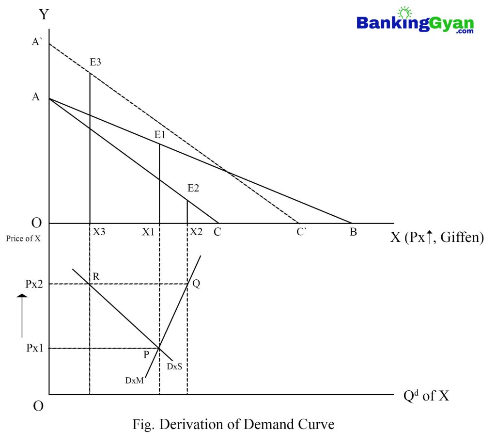
Derivation of demand curve for Giffen good when Price increase using RPT (Figure only)
Derivation of Indifference Curve Using RPT
The Revealed Preference Theory (RPT) does not need any indifference curve for consumer behavior analysis and demand curve derivation but if required IC can be derived and also we can proof the CONVEXITY of the IC using this theory. It means we can derive an Indifference Curve by observing the actual behavior of the consumer in the real market and can also proof such IC is convex to the origin.
In order to derive the IC, we have to observe the consumer’s choice in the market under different prices of the commodities X and Y.
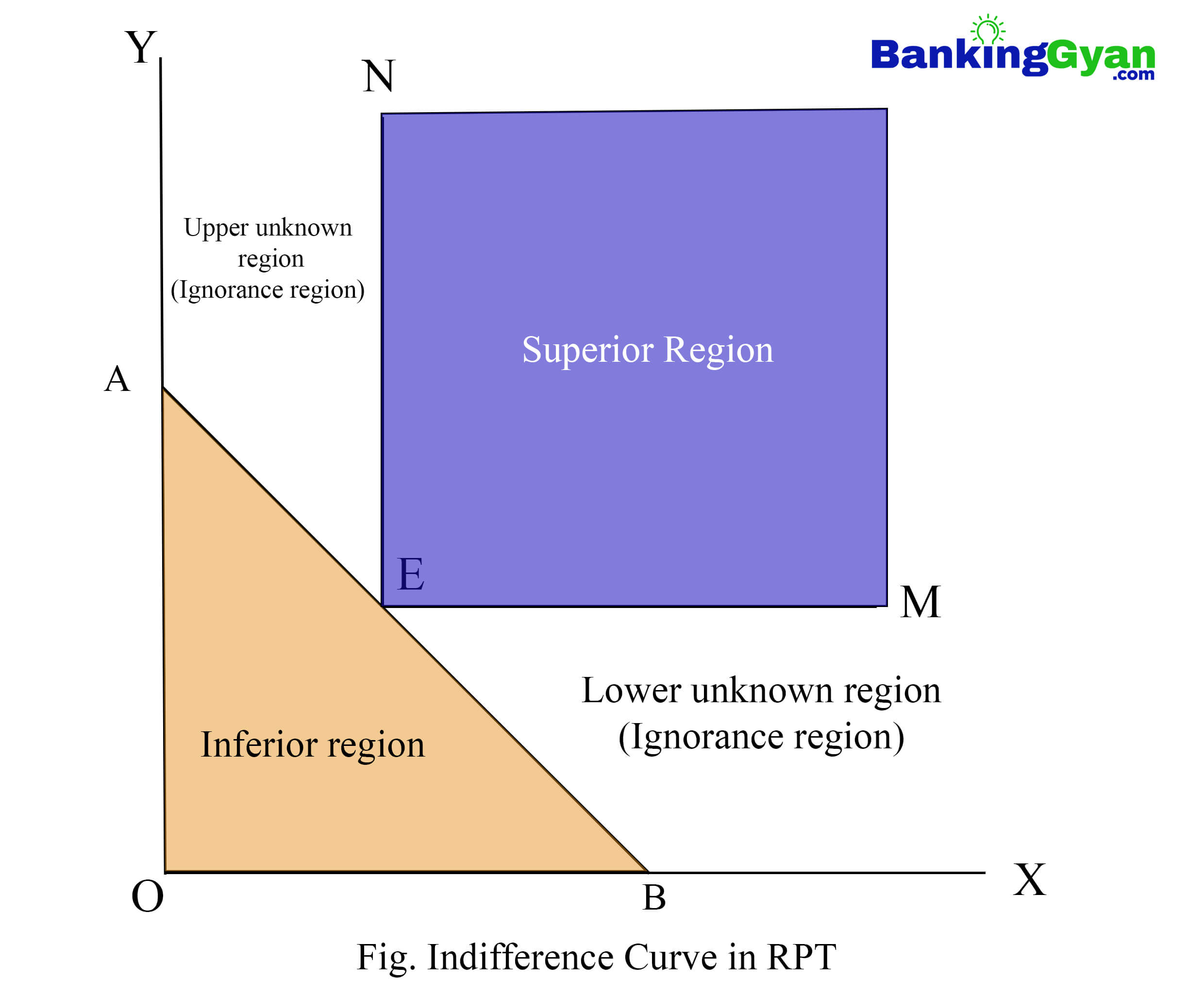
Here, AB is the initial budget line and so the consumer can select any bundle on this budget lines or below. Assume that the consumer is observed to be selecting E bundle which means the rest of the other bundle on this budget line AB or below of it are inferior to the selected bundle E. So, area AOB (shown in orange color) represents the inferior region to the bundle E. Now, let’s draw NE perpendicular EM and the area covered by NEM represents the superior region to E because any combination in this contains more quantity of either X or Y or both.
The area enclosed by NEB contains more quantity of X but less quantity of Y then the bundle E. And so the utility represented by any bundle on this area may be higher, lower or equal to the utility given by bundle E.
Similarly, the area AEN is the upper unknown region which means this area has more, less of equal utility than bundle E. The IC representing the utility given by bundle E does not pass into the inferior and superior region and so it should pass through the unknown region.
Since in the unknown region some bundles give more satisfaction or superior to bundle E, some give less satisfaction or inferior to bundle E, and some give equal satisfaction or indifference to bundle E. So, in order to derive IC representing the utility given by bundle E, we have to minimize both unknown region by increasing the superior and inferior region in such a way that it is possible to locate the perfect IC.
In order to minimize the unknown region, we have to observe the consumer’s choice in the real market under the different prices of X and Y.
For this, consider the price of X declines and price of Y increases at the same time. So that the new budget lines is A`B` as shown in the figure below.

Under this new budget line A`B`, the consumer does not select any bundle on the segment A`E1 as it is already in the inferior region. So, the consumer can select any bundle E1B`. Assume that, the consumer is found to be selecting bundle E1.Which means the area ΔBE1B`is revealed to be inferior to E1.
- i.e. E1 > ΔBE1B` (New budget line)
- E > E1 (Initial Budget line)
- E > ΔBE1B` (From transitivity property)
This means, ΔBE1B`is inferior to E which means we are able to minimize the lower unknown (Ignorance region) by ΔBE1B`.
Now, assume that the price of X increases and price of Y declines such that new budget line A“B“ is formed. In this new budget line the consumer does not select any bundle on E2B“ because it is already in the inferior region.
The consumer is found to be selecting E2 which means
- i.e. E2 > ΔAE2A“(New budget line)
- E > E2 (Initial Budget line)
- E > ΔAE2A“(From transitivity property)
This shows that we are able to minimize the upper unknown region by ΔAE2A“. If we repeat same process under various prices of X and Y, we are able to minimize unknown region and help to locate the area through which the IC representing the utility given by bundle E and pass through as shown in the figure above.
Convexity of Indifference Curve Using RPT
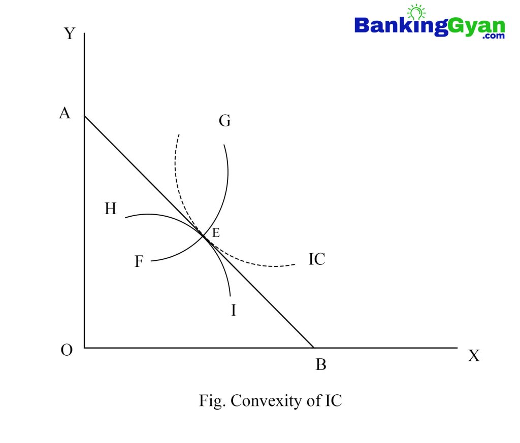
Here, the IC passing through E can not be a downward sloping straight line AB because by choosing bundle E rest of the other bundle on the budget line AB are revealed to be inferior.
Similarly, the IC passing through E can not be upward sloping curve as FG because the part below E is in inferior region and the part above E is in superior region.
Again, the IC passing through E can not be a concave curve HI because all of it is lies within the inferior region. So, only the possible shape us CONVEX SHAPE shown by IC. It means the indifference curve derived by using the Revealed Preference Theory (RPT) is convex to the origin.