Equilibrium = It is the state of rest, which means no tendency to change.
A consumer is said to be in equilibrium if s/he has maximized utility under the given constraints. To explain the consumer’s equilibrium, assume that there are two commodities, X and Y, with respective prices of Px and Py.
Let M be the given money income
Objective: Max U = f(x,y) subject to M = PxY + PyY
In this case, the consumer attains equilibrium by spending the given income M between X and Y in such a way that the utility given by them is maximum.
The utility given by X and Y is assumed to be represented by the usual shape of an Indifference Curve (IC), which is downward sloping and convex to the origin. Then, the consumer is said to maximize the utility if the following two conditions are satisfied simultaneously.
First order/primary/necessary condition
Slope of IC = Slope of budget line

Second order/secondary/sufficient condition
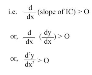
The IC must be convex to the origin at the point of tangent with the budget line. For convexity, the rate of change of the slope of IC must be positive.
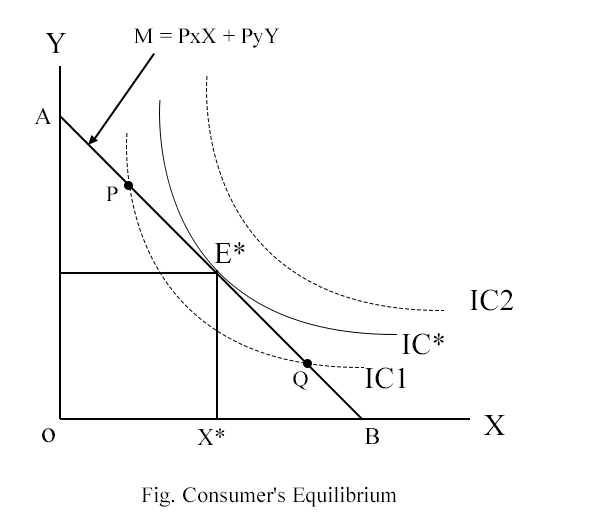
Here, AB is the given budget line and IC1, IC*, and IC2 are indifference curves, respectively. Different levels of utility given by X and Y to the consumer are shown by IC*, IC1, and IC2. In the figure, IC2 represents the higher level of utility, and so it is represented by the consumer, but under the given budget, it is unattainable.
Under the given budget, IC1 and IC* levels of satisfaction are attainable, but the consumer prefers the IC* level of satisfaction because it is higher than the IC1. As both of the conditions of utility maximization are satisfied at E*, the consumer attains equilibrium at E* by consuming OX* quantity of X and OY* quantity of Y. This gives the highest possible level of utility IC* under the given budget.
Therefore, a consumer is said to be in equilibrium when s/he maximizes utility under the given budget, and such utility is said to be at a maximum at a point where the slope of the IC and the budget line are equal.
Effect of Change in Income of Consumer
खरिदकर्ताको आयमा भएको परिवर्तनले पार्ने असर
उदाहरण
- जम्मा पैसा = रु. १०००
- स्याउ = रु. १०० प्रति केजी
- आँप = रु. २०० प्रति केजी
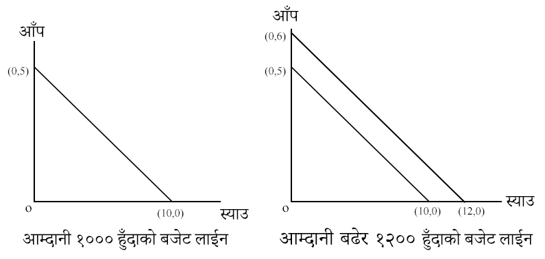
- When income increases → Budget line shifts outward
- When income decreases → Budget line shifts inward
→ If the income of the consumer changes, other things remaining the same, it seems that the budget line shifts outward and inward if income decreases.
→ This affects the consumer’s equilibrium, called the income effect.
→ Income effect is positive for normal commodities and negative for inferior commodities.
- For normal IE>0, if Income↑, Qd↑ or if Income↑, Qd↓
- For inferior goods IE <0, if Income↓, Qd↑ or if Income↑, Qd↓
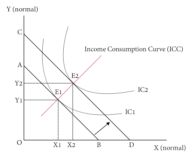
Here, AB is the initial budget line in which the consumer attains equilibrium at E1 with OX1 quantity of X and OY1 quantity of Y. When the income of a consumer increases. The budget line shifts outward from AB to CD, then the consumer attains a new equilibrium at E2 with OX2 quantity of X and OY2 quantity of Y. This shows that if income increases, the consumer consumes more quantity of X and Y.
Which means both X and Y are normal to the consumer.
If we join different equilibrium points that arose due to the change in income with origin, we get the Income Consumption Curve (ICC). i.e., The Icc will be upward sloping, which implies a positive income effect on both commodities.
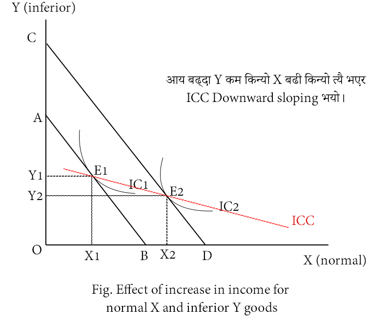
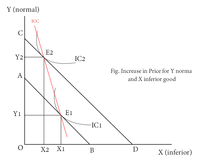
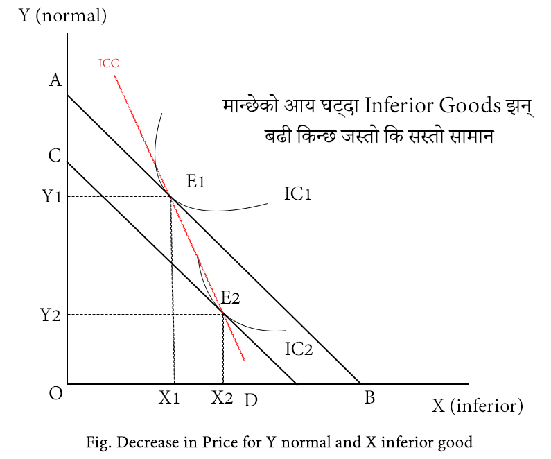
If any of the commodities is inferior, then the ICC bends towards the axis of normal, implying a negative income effect for inferior and a positive income effect for normal as shown in the figure below.
Effect of Change in Price of the Commodity
If the price of the commodity changes, things remaining the same, it swings the budget line outward (if the price decreases) and inward (if the price increases). Such swings in the budget line affect the equilibrium quantity of the commodity, which is known as the price effect.
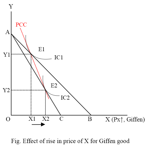
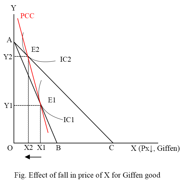
Such a price effect is negative for normal goods and positive for Giffen goods.
- For normal PE < 0 ———– If P ↑⇒Qd↓ and P↓ ⇒ Qd ↑
- For giffen PE > 0 ———– If P ↑⇒Qd↑ and P↓ ⇒ Qd ↓
Effect of the price fall of X (normal good)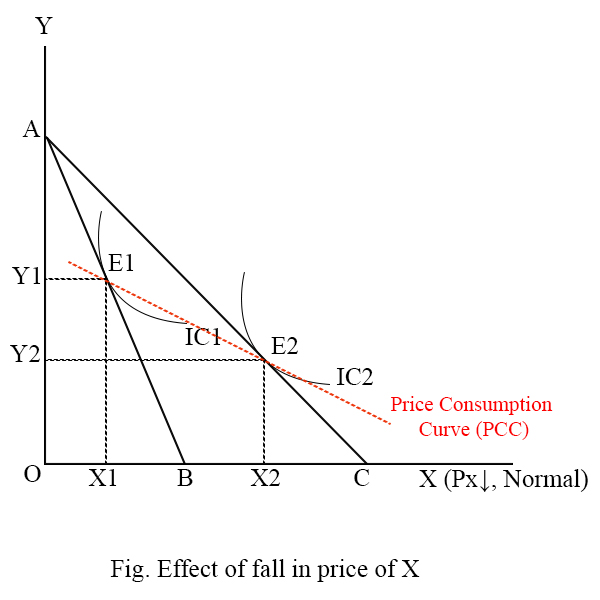
Here, the consumer is in equilibrium at E1 with OX1 quantity of X. Now, assume that the price of X declines, and so the budget line swings outward from AB to AC, and the consumer’s equilibrium is attained at E2 with OX2 quantity of X. This movement from E1 to E2 is due to the price effect. i.e.
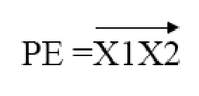
Now, if we join these two equilibrium points, E1 and E2, we get the Price Consumption Curve (PCC). Which may be downward-sloping, upward-sloping, +ve sloping, -ve sloping, or parallel to the axis of the commodity. This all depends on the price elasticity of demand.
Effect of the price fall of X (Giffen good)
Effect of the price rise of X (Giffen good)